3.1 Category 1 Variable 1: White Population

[Map]

popupLabels_white <- paste0("<b>",countyGIS_map$name," (",countyGIS_map$FIPS,")</b>",
                    "<br><font color='",countyGIS_map$FontColorWinner,"'>",countyGIS_map$winner, 
                    ": ",
                    format(countyGIS_map$pctWinner*100,digits=4, trim=TRUE),
                    "%</font>",
                    "<br>Total votes: ", format(countyGIS_map$totalVotes,big.mark=",", trim=TRUE),
                    "<br>Percent White: ", format(round(countyGIS_map$pct_white, 2),big.mark=",", trim=TRUE),
                    "%</font>"
                    ) %>% 
              lapply(htmltools::HTML)

pal <- colorBin("Greys", countyGIS_map$pct_white,bins = c(0, 20, 40, 60, 80, 100), reverse=TRUE)


leaflet(countyGIS_map, options = leafletOptions(crsClass = "L.CRS.EPSG3857"), width="100%") %>%
  addPolygons(weight = 0.5, color = "gray", opacity = 0.7,
    fillColor = ~pal(pct_white), fillOpacity = 1, smoothFactor = 0.5,
    label = popupLabels_white,
    labelOptions = labelOptions(direction = "auto")) %>%
    addPolygons(data = stateGIS,fill = FALSE,color="black",weight = 1) %>%
    addLegend(pal = pal,values = ~countyGIS_map$pct_white, opacity = 0.7, title = "% White",position = "bottomright")

[Scatter plot]

pct_white_vs_pctGOP <- ggplot(countyGIS_stat, aes(pct_white, pctGOP)) + 
  geom_point(aes(alpha = pct_white, shape = ".")) + 
  geom_smooth(method = "lm", se = FALSE) 

pct_white_vs_pctGOP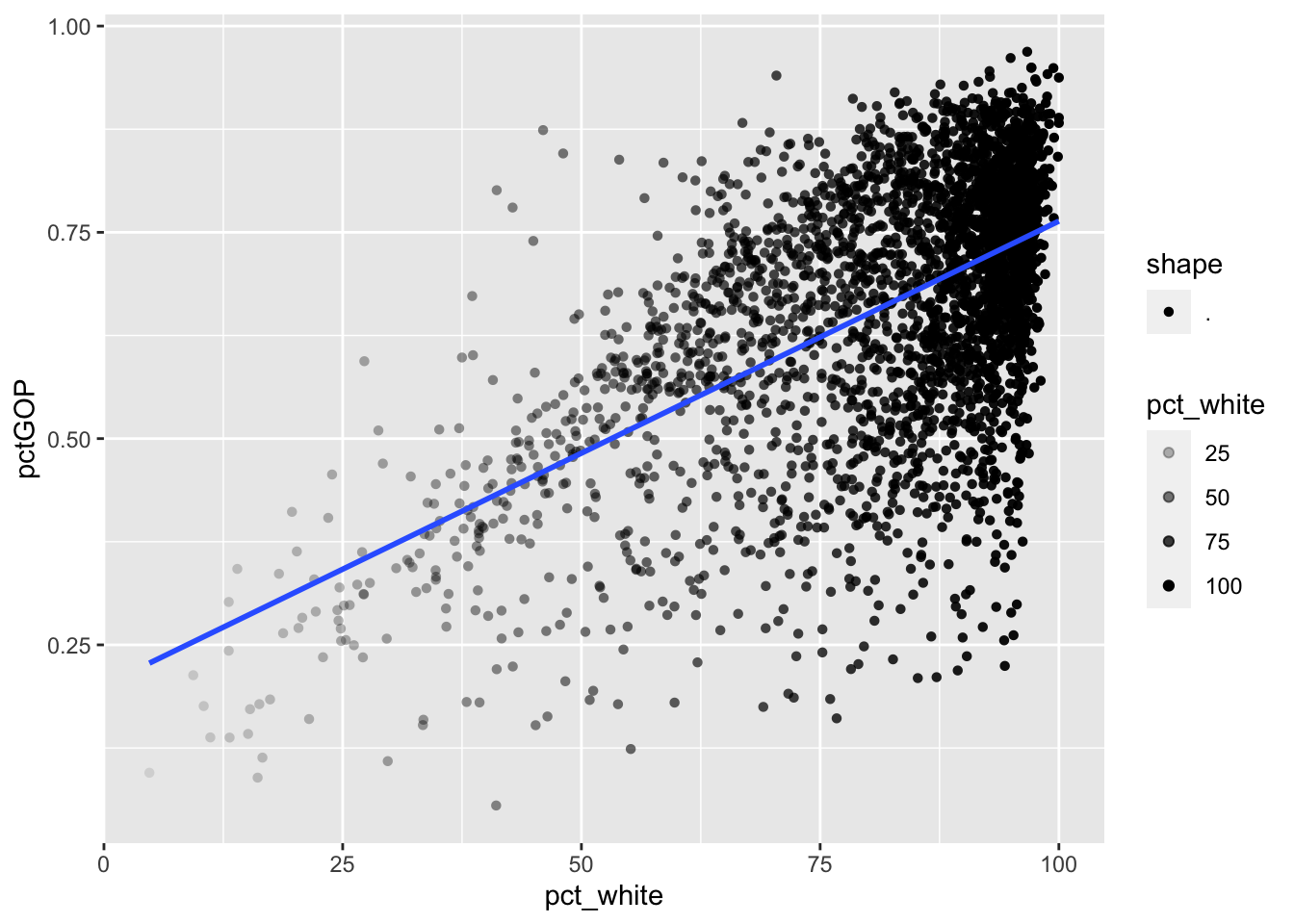

[Regression]

# Estimate regression model
pct_white_reg <- lm(pctGOP ~ pct_white, data=countyGIS_stat)

# Display model results
pander(summary(pct_white_reg))

	Estimate	Std. Error	t value	Pr(>|t|)
(Intercept)	0.2011	0.01214	16.57	4.122e-59
pct_white	0.005625	0.0001448	38.85	4.965e-269

Fitting linear model: pctGOP ~ pct_white

Observations	Residual Std. Error	\(R^2\)	Adjusted \(R^2\)
3083	0.1321	0.3288	0.3286